Foundations of AI and ML
Content
Lisam
Course materials
/
Section
Model Evaluation: A Classification Example
Introduction
Selecting the best-performing model for a specific application is not always a straightforward task. Most often, we need to employ some type of validation strategy to avoid issues such as over- and underfitting. In this problem, we will focus on the task of selecting a binary classification model using a separate validation set.
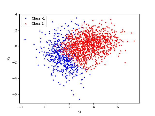
We consider a synthetic data set, shown in the figure below. The two classes are labeled as “-1” and “1”, respectively. The training data consist of 1640 observations with 472 observations from class -1 and the rest from class 1.

Three logistic regression models have been trained on this data, using the scikit-learn library. All of the models predict the probability that an input $\mathbf{x}$ belongs to class 1 according to a standard logistic regression model
What differs between the three models is their complexity; the dimension of the model parameters $\boldsymbol{\theta}$ (and the dimension of the input).
The first model is the simplest one. It predicts the class probability based only on the original features $x_1$ and $x_2$, so
and $\boldsymbol{\theta}$ has dimension 3.
For the other two models, we have added polynomial features to the input vector, as described in the linear regression example in the previous section. The second model makes its predictions based on the original features as well as on second order terms. We replace $\mathbf{x}$ with $\mathbf{\tilde{x}}$ in the equation above, where
This model has six parameters in total, one for each element of the feature vector above, i.e. the dimension of $\boldsymbol{\theta}$ is 6.
The input to the last model is a forth order polynomial,
and, consequently, the dimension of $\boldsymbol{\theta}$ is 15.
Let us have a look at the decision boundaries of the three models.

We have introduced the models in order of their complexity. In general, more complex models are also more flexible. In this case, we can see that while the first model has a linear decision boundary, the decision boundary of the last model is able to adapt more to the non-linear patterns in the training data. The second model, with a quadratic decision boundary, is somewhere in between.
Your task is to evaluate the three models in order to try to figure out which model is the best choice given the problem at hand. You will start by calculating the training error, or the misclassification rate, of each model.
Question A: Misclassification Rate
The code shown below loads the three models considered as well as the data that was used to train them. The misclassification_rate function takes as input an input data array,
true class labels and a model. Fill in the empty lines in the function so that it returns the misclassification rate (see Eq. 4.1 in the course book) of the model on the given data. Run the code to calculate, for each model,
the error on the training data.
Question B: Smallest Training Error
Which model has the smallest training error?
Error on Validation Data
Apart from the training data, you also have an extra hold-out validation data set of 411 observations at your disposal. Let’s look at the model errors on this new dataset.
Run the code below to calculate the validation error of each model using the function from Question B.
Question C: Smallest Validation Error
Based on the output of the code, which model has the smallest validation error?
Is the model with the smallest validation error the same as the one that had the smallest error on the training data?
Question D: Selecting a Model
You want to select a model that performs well on new data. Based on the full analysis that you have done, which model should you choose as the final model?
Conclusion
Well done with the model selection and evaluation! Using a hold-out validation dataset we could evaluate the generalization performance of the models. We concluded that, among the the three candidate models, the second one was the most appropriate choice for this particular data, despite having slightly larger training error than the third model. In this example, we could perhaps have drawn the same conclusion directly by looking at the plots of the decision boundaries for the three models. However, drawing such plots is not possible in most practical applications, when the dimension of $\mathbf{x}$ is larger than two. The validation approach, on the other hand, is applicable regardless of the input dimension!
You might have observed in this example that the dataset was slightly imbalanced, with observations from class 1 constituting around 70% of the data. This slight data imbalance probably did not have a very large effect on the model performance, considering also that the problem was relatively simple. Had the larger class been even bigger, we might have wanted to somehow account for the data imbalance to counteract possible negative effects on the performance of the final model. This is something that we will explore in more detail in the next exercise.
This webpage contains the course materials for the course TDDE56 Foundations of AI and Machine Learning.
The content is licensed under Creative Commons Attribution 4.0 International.
Copyright © 2022 Linköping University